Our Methods
Our commercial methods build on the success of many years of combined brain research and software development at the University of Iowa. We are authorized to modify and use BRAINS to provide brain morphometry as a commercial service, and are indebted to all the researchers who have contributed to their efforts. Our commercial extension of these methods, including highly accurate, new applications of the artificial neural network (ANN) subcortical parcellations, is contributed back to their laboratories to enhance their ongoing efforts.
But everyone is using something else. How good are you?
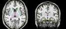
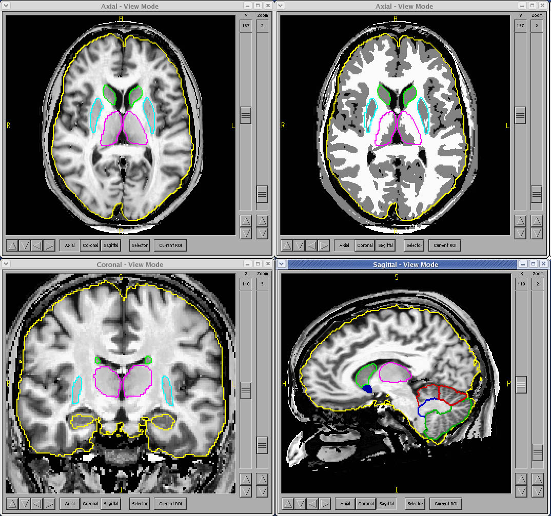
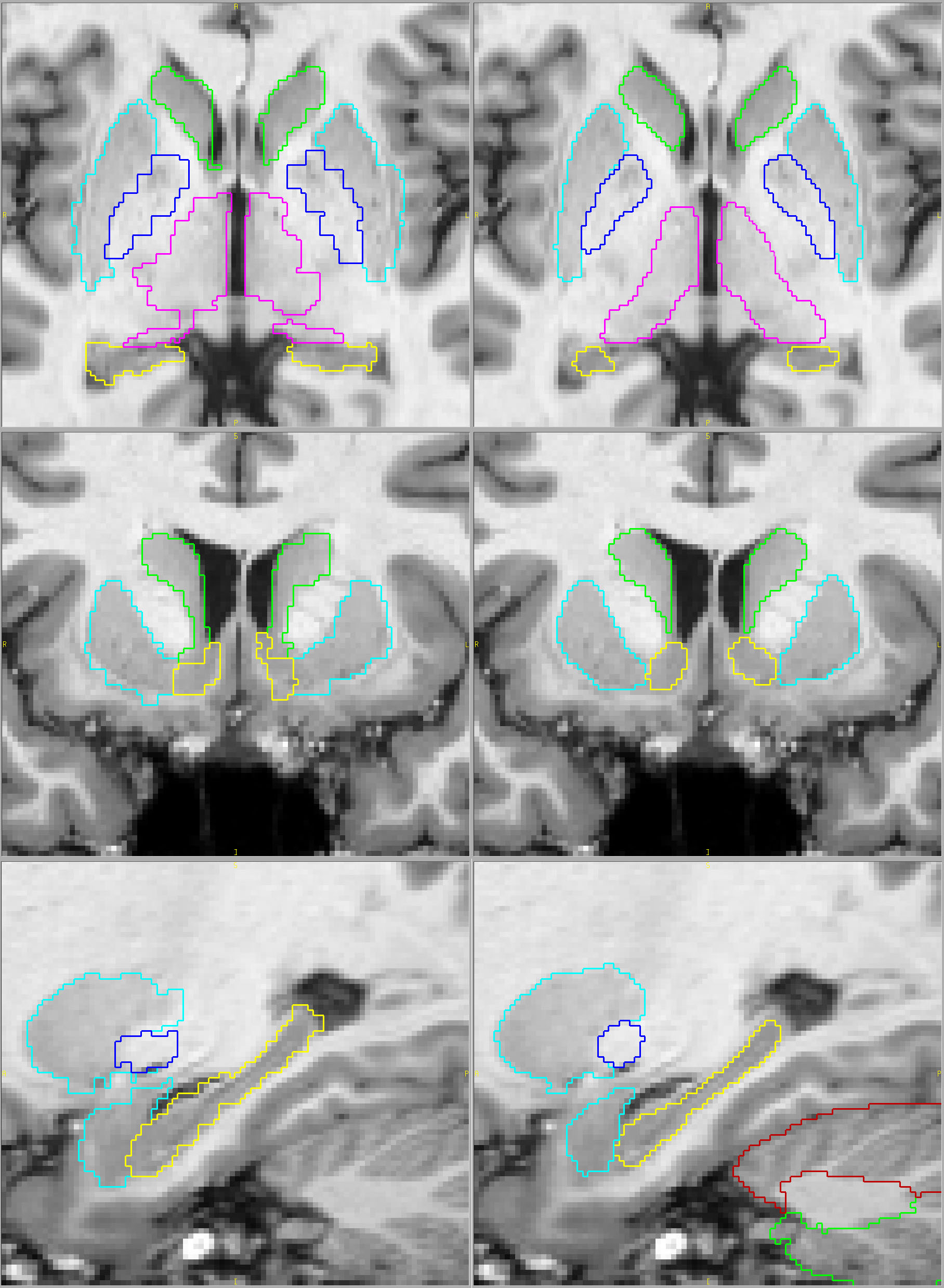
Compare below the most popular fully automated method on the left with our results on the right (click on the pictures for full-sized views). You tell us. Which parcellation looks more valid? Does your putamen measure include external capsule, claustrum and extreme capsule? Do you want your hippocampus measures to include alveus, choroid plexus and other surrounding white matter?
Their results Our results
Background
BRAINS software is a product of over 2 decades of development at the University of Iowa Department of Psychiatry. Primary development was completed by Dr. Nancy Andreasen's research group.
http://www.psychiatry.uiowa.edu
Current development is led by Dr. Vincent Magnotta in the Department of Radiology, with hosting of the source code and binaries at:
http://www.nitrc.org/projects/brains/
BRAINS has a long history of adherence to strict requirements of reliability, accuracy and validity.
No classification priors needed
Tissue classification in the BRAINS workup is accomplished through use of a discriminant classification method. Discriminant functions are created through use of known intensities of each pure tissue type for each subject. These functions are then used to determine the likelihood of a voxel being GM vs. WM or GM vs. CSF. This produces a 3D continuous-classified tissue image. To avoid any ambiguity each voxel may then be discretely classified as purely one tissue type.
The algorithm begins by randomly sampling pure tissue throughout the brain region with selection of points randomly within the brain, resulting in thousands of random samples of tissue. Each voxel will be assigned a label of GM, WM or CSF, but if it is to be representative of pure tissue intensities, each plug must be pure. To evaluate the purity of each plug, the variance of the intensities of 8 voxels around each plug is calculated. If the variance is sufficiently small the plug is assumed to be pure, containing voxels of only one tissue type.
The plugs are then sorted into tissue types based on their intensities in each modality (T1, T2 and PD if available) by use of k-means clustering, creating a pure training set for each of the tissue types. Discriminant functions based on these training sets then classify each voxel in the image.
The clear advantage of this method is that it doesn't depend on how well your subject's morphometry matches that of the template brain and priors used by so many other methods. Dependence on priors can result in loss of the ability to capture the naturally occuring variability you are trying to measure. And, if you are working with entire populations that are non-standard, such as children, elderly, or those with significant atrophy, the effect may be even more accentuated.
Precision Brain Morphometry
Throughout Development
Throughout the development of BRAINS workup methods the reference for each step has been manually defined by experienced human raters. The first example is the tissue classification algorithm. Manual raters traced each of the tissue types completely on numerous slices on a sample of scans. The classification of the discriminant method was then compared to that of the manual raters. As segmentation methods were automated through use of artificial neural networks, the training was completed on a set of manually traced structures, and tested on manually traced structures from a completely different set of scans, ensuring that the training was based on accurate exemplars and that it was also broadly applicable to scans different from those in the training set.
The testing of these methods generally is accomplished to satisfy three criteria: reliability, accuracy and validity.
Reliability refers to the reproducibility of the measures. The concept has its roots in concerns that raters in cognitive testing should be, if possible, interchangeable. That is, that the results of the testing should be the same no matter who is rating a subject. In addition to ensuring human raters are interchangable, it is also important when developing automated methods – the automated method should produce measures that can be interchangeable with the manual measures. The numerical process used to calculate reliability is to include measures by both methods on a sample of subjects (usually 15-30 subjects), perform an analysis of variance with some algorithm such as restricted maximum likelihood or a more rigorous ANOVA. The reliability, expressed as intraclass correlation (R2) is defined as the ratio of the variance due to subject divided by the variance due to all sources, including error. This ranges from 0 to 1, with acceptable numbers ranging from 0.75 to 0.99, depending on the structure or measure. For instance, large structure such as the intracranial volume (ICV) should be measured quite reliably, with icc (R2) typically being > 0.99. For small structures such as the nucleus accumbens, where the edge voxels (where the errors are made) compose a relatively large proportion of the volume, an ICC of 0.8 between two manual raters would be considered quite good.
Accuracy refers to how similar measures are, and is generally determined by a comparison between the two raters or methods means and some measure of distribution, such as standard deviation or variance. Depending on the structure being measured, a difference of more than a few percent would suggest that the measures are not accurately reflecting the “true” volume.
Validity, in brain imaging, has two meanings. First, we need to have an expert verify that we are indeed measuring the structure we intend to. As part of the methods development process traces of each structure are reviewed by a neuroanatomist to establish that the method is indeed measuring the correct structure, including all the correct nuclei, and excluding other structures. In a more objective sense, validity refers to whether the two tracers or methods are “seeing” the same structure based on their actual traces. It is measured by overlap, or intersection/union. This additional qualification ensures that the two methods/tracers are actually measuring the same thing. Here is an extreme example to clarify this point. Let’s say Rater 1 traces caudates correctly. Tracer 2 reverses the names on the saved traces, switching left and right. Since the left and right caudate for a given subject really don’t vary much compared to how much they vary between subjects, their measures may be quite reliable and numerically accurate, but the traces are completely invalid. Overlap catches this, and their overlap would be 0. A less obvious example would be parcellation of the cerebellum. One rater chooses lobe VI correctly, following the primary fissure and superior posterior fissues to delineate it from the rest of the cerebellum. In some scans, the other rater misses by a single folia in the lateral regions (where folia can split or combine to create different, complicated patterns). Their volumes may be very similar, the reliability will be good, and only through calculation of overlap will one have an objective measure of their differences.
The reliability, accuracy and validity measures used by the researchers in Dr. Andreasen’s lab, and in general those at Iowa, were strictly inter-rater, not intra-rater. For a rater to do the same as he/she just did on the same scan on the day before only proves that they can see something themselves. It doesn’t show that the method can be learned by others, or that there is any agreement as to the structure’s definition. Just that one person is uniquely able to produce measures that are consistent with themselves. At least two traces really need to be able to apply a method to establish that the method can be replicated, and maybe that it is a bit more valid that two people agree on the borders in a consistent way. Not only is it important that methods be able to be replicated within and across labs, but in establishing reliability there can be no do-overs – once two tracers have used a set of scans for a comparison of their work, but have had problems in establishing reliability, they must relearn the method and apply it to a completely new set of scans – otherwise you again risk simply memorizing how you both agreed or disagreed, and you do not show a broader applicability of the methods, training and skills to new scans. Numerous publications can be found where either a single rater completes tracing on a set of scans numerous times, repeating the traces until their work is consistent. That does not prove much about the quality of their work, they simply got to know the set of scans well enough to trace consistent with their own mistakes. This is an extremely important point, as you cannot assume that these tracers will approach a new set of scans in the same way.
In addition to these measures, it is important that there is a consistency to these skills in the lab. It is not easy to learn a structure, and to lose a technician who is the gold standard for a structure makes it difficult to maintain continuity. At Iowa they have had a long history of high-quality, consistent staff.
How Does This Create Better
Automated Methods?
The artificial neural network methods used in BRAINS software have developed over time from a relatively crude way to have a starting point for editing a structure, to a high-performance algorithm that can produce reliable, accurate and valid parcellations of caudate, putamen, globus, thalamus, accumbens, hippocampus and cerebellum, with a success rate of over 90% for most structures. An important part of the input to the ANN is a probability map for where to find each structure. These probability maps are generated from the manually traced structures. Using a high-dimensional nonlinear warping algorithm, these probability maps are registered to the data sets. Next, the artificial neural network is trained on the manual parcellations to learn the finer details at the edges of the structures. It is this learning based on the manual parcellations that gives the ANN method a distinct edge over others.
Finally, the trained ANN is tested on a different set of scans to assess its reliability, accuracy and validity compared to manual raters. This ensures it will operate on a par with a set of technicians.
Why Are Technicians Even Needed?
We don't subscribe to a policy of "run it through and use it." Would you want a mechanic who doesn't check the torque on your lug nuts after changing a tire? Would you want a surgeon who doesn't count the sponges before closing you up? We wouldn't, and we know you wouldn't want that kind of sloppiness in your research, either.
At Brain Image Analysis each scan is carefully reviewed after processing, and those scans with tissue classifications or parcellations that are inadequate are set aside for manual intervention. It takes a trained eye to assess these issues, and our technicians have an average of over 10 years experience in the field. For those with tissue classification issues, there generally are artifacts that need to be reviewed and cleared up before reprocessing. For those with parcellation errors, the solution is often to manually edit the structures, correcting those areas that are inaccurate. Generally less than 5% of good quality scans require any followup attention, but we are sure you will agree that your research is worth getting it right.